Probability Distribution | Formula, Types, & Examples
A probability distribution is a mathematical function that describes the probability of different possible values of a variable. Probability distributions are often depicted using graphs or probability tables.
| Outcome | Probability |
|---|---|
| Heads | Tails |
| .5 | .5 |
Common probability distributions include the binomial distribution, Poisson distribution, and uniform distribution. Certain types of probability distributions are used in hypothesis testing, including the standard normal distribution, Student’s t distribution, and the F distribution.
Table of contents
What is a probability distribution?
A probability distribution is an idealized frequency distribution.
A frequency distribution describes a specific sample or dataset. It’s the number of times each possible value of a variable occurs in the dataset.
The number of times a value occurs in a sample is determined by its probability of occurrence. Probability is a number between 0 and 1 that says how likely something is to occur:
- 0 means it’s impossible.
- 1 means it’s certain.
The higher the probability of a value, the higher its frequency in a sample.
More specifically, the probability of a value is its relative frequency in an infinitely large sample.
Infinitely large samples are impossible in real life, so probability distributions are theoretical. They’re idealized versions of frequency distributions that aim to describe the population the sample was drawn from.
Probability distributions are used to describe the populations of real-life variables, like coin tosses or the weight of chicken eggs. They’re also used in hypothesis testing to determine p values.
The farmer weighs 100 random eggs and describes their frequency distribution using a histogram:
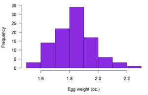
She can get a rough idea of the probability of different egg sizes directly from this frequency distribution. For example, she can see that there’s a high probability of an egg being around 1.9 oz., and there’s a low probability of an egg being bigger than 2.1 oz.
Suppose the farmer wants more precise probability estimates. One option is to improve her estimates by weighing many more eggs.
A better option is to recognize that egg size appears to follow a common probability distribution called a normal distribution. The farmer can make an idealized version of the egg weight distribution by assuming the weights are normally distributed:
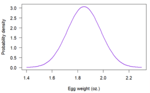
Since normal distributions are well understood by statisticians, the farmer can calculate precise probability estimates, even with a relatively small sample size.
Variables that follow a probability distribution are called random variables. There’s special notation you can use to say that a random variable follows a specific distribution:
- Random variables are usually denoted by X.
- The ~ (tilde) symbol means “follows the distribution.”
- The distribution is denoted by a capital letter (usually the first letter of the distribution’s name), followed by brackets that contain the distribution’s parameters.
For example, the following notation means “the random variable X follows a normal distribution with a mean of µ and a variance of σ2.”

There are two types of probability distributions:
Discrete probability distributions
A discrete probability distribution is a probability distribution of a categorical or discrete variable.
Discrete probability distributions only include the probabilities of values that are possible. In other words, a discrete probability distribution doesn’t include any values with a probability of zero. For example, a probability distribution of dice rolls doesn’t include 2.5 since it’s not a possible outcome of dice rolls.
The probability of all possible values in a discrete probability distribution add up to one. It’s certain (i.e., a probability of one) that an observation will have one of the possible values.
Probability tables
A probability table represents the discrete probability distribution of a categorical variable. Probability tables can also represent a discrete variable with only a few possible values or a continuous variable that’s been grouped into class intervals.
A probability table is composed of two columns:
- The values or class intervals
- Their probabilities
| Greeting | Probability |
|---|---|
| “Greetings, human!” | .6 |
| “Hi!” | .1 |
| “Salutations, organic life-form.” | .2 |
| “Howdy!” | .1 |
Notice that all the probabilities are greater than zero and that they sum to one.
Probability mass functions
A probability mass function (PMF) is a mathematical function that describes a discrete probability distribution. It gives the probability of every possible value of a variable.
A probability mass function can be represented as an equation or as a graph.
The probability mass function of the distribution is given by the formula:

Where:
 is the probability that a person has exactly
  sweaters
 is the mean number of sweaters per person (
 , in this case)
 is Euler’s constant (approximately 2.718)
 is the probability that a person has exactly
  sweaters
 is the mean number of sweaters per person (
 , in this case)
 is Euler’s constant (approximately 2.718)
This probability mass function can also be represented as a graph:
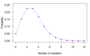
Notice that the variable can only have certain values, which are represented by closed circles. You can have two sweaters or 10 sweaters, but you can’t have 3.8 sweaters.
The probability that a person owns zero sweaters is .05, the probability that they own one sweater is .15, and so on. If you add together all the probabilities for every possible number of sweaters a person can own, it will equal exactly 1.
Common discrete probability distributions
| Distribution | Description | Example |
|---|---|---|
| Binomial | Describes variables with two possible outcomes. It’s the probability distribution of the number of successes in n trials with p probability of success. | The number of times a coin lands on heads when you toss it five times |
| Discrete uniform | Describes events that have equal probabilities. | The suit of a randomly drawn playing card |
| Poisson | Describes count data. It gives the probability of an event happening k number of times within a given interval of time or space. | The number of text messages received per day |

Continuous probability distributions
A continuous probability distribution is the probability distribution of a continuous variable.
A continuous variable can have any value between its lowest and highest values. Therefore, continuous probability distributions include every number in the variable’s range.
The probability that a continuous variable will have any specific value is so infinitesimally small that it’s considered to have a probability of zero. However, the probability that a value will fall within a certain interval of values within its range is greater than zero.
Probability density functions
A probability density function (PDF) is a mathematical function that describes a continuous probability distribution. It provides the probability density of each value of a variable, which can be greater than one.
A probability density function can be represented as an equation or as a graph.
In graph form, a probability density function is a curve. You can determine the probability that a value will fall within a certain interval by calculating the area under the curve within that interval. You can use reference tables or software to calculate the area.
The area under the whole curve is always exactly one because it’s certain (i.e., a probability of one) that an observation will fall somewhere in the variable’s range.
A cumulative distribution function is another type of function that describes a continuous probability distribution.

Where:
 is the probability density of egg weight
 is the mean egg weight in the population (
 oz., in this case)
 is the standard deviation of egg weight in the population (
 oz., in this case)
 is the probability density of egg weight
 is the
  oz., in this case)
 is the
  oz., in this case)
The probability of an egg being exactly 2 oz. is zero. Although an egg can weigh very close to 2 oz., it is extremely improbable that it will weigh exactly 2 oz. Even if a regular scale measured an egg’s weight as being 2 oz., an infinitely precise scale would find a tiny difference between the egg’s weight and 2 oz.
The probability that an egg is within a certain weight interval, such as 1.98 and 2.04 oz., is greater than zero and can be represented in the graph of the probability density function as a shaded region:
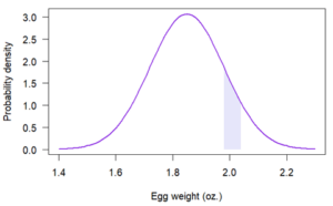
The shaded region has an area of .09, meaning that there’s a probability of .09 that an egg will weigh between 1.98 and 2.04 oz. The area was calculated using statistical software.
Common continuous probability distributions
| Distribution | Description | Example |
|---|---|---|
| Normal | Describes data with values that become less probable the farther they are from the mean, with a bell-shaped probability density function. | SAT scores |
| Continuous uniform | Describes data for which equal-sized intervals have equal probability. | The amount of time cars wait at a red light |
| Log-normal | Describes right-skewed data. It’s the probability distribution of a random variable whose logarithm is normally distributed. | The average body weight of different mammal species |
| Exponential | Describes data that has higher probabilities for small values than large values. It’s the probability distribution of time between independent events. | Time between earthquakes |
How to find the expected value and standard deviation
You can find the expected value and standard deviation of a probability distribution if you have a formula, sample, or probability table of the distribution.
The expected value is another name for the mean of a distribution. It’s often written as E(x) or µ. If you take a random sample of the distribution, you should expect the mean of the sample to be approximately equal to the expected value.
- If you have a formula describing the distribution, such as a probability density function, the expected value is usually given by the µ parameter. If there’s no µ parameter, the expected value can be calculated from the other parameters using equations that are specific to each distribution.
- If you have a sample, then the mean of the sample is an estimate of the expected value of the population’s probability distribution. The larger the sample size, the better the estimate will be.
- If you have a probability table, you can calculate the expected value by multiplying each possible outcome by its probability, and then summing these values.
| Eggs | Probability |
|---|---|
| 2 | 0.2 |
| 3 | 0.5 |
| 4 | 0.3 |
What is the expected value of robin eggs per nest?
Multiply each possible outcome by its probability:
| Eggs (x) | Probability (P(x)) | x * P(x) |
|---|---|---|
| 2 | .2 | 2 * 0.2 = 0.4 |
| 3 | .5 | 3 * 0.5 = 1.5 |
| 4 | .3 | 4 * 0.3 = 1.2 |
Sum the values:
E(x) = 0.4 + 1.5 + 1.2
E(x) = 3.1 eggs
The standard deviation of a distribution is a measure of its variability. It’s often written as σ.
- If you have a formula describing the distribution, such as a probability density function, the standard deviation is sometimes given by the σ parameter. If there’s no σ parameter, the standard deviation can often be calculated from other parameters using formulas that are specific to each distribution.
- If you have a sample, the standard deviation of the sample is an estimate of the standard deviation of the population’s probability distribution. The larger the sample size, the better the estimate will be.
- If you have a probability table, you can calculate the standard deviation by calculating the deviation between each value and the expected value, squaring it, multiplying it by its probability, and then summing the values and taking the square root.
| Eggs (x) | Probability (P(x)) | x – E(x) |
|---|---|---|
| 2 | .2 | 2 − 3.1 = −1.1 |
| 3 | .5 | 3 − 3.1 = −0.1 |
| 4 | .3 | 4 − 3.1 = 0.9 |
Square the values and multiply them by their probability:
| Eggs (x) | Probability (P(x)) | x – E(x) | [x – E(x)]2 * P(x) |
|---|---|---|---|
| 2 | .2 | 2 − 3.1 = −1.1 | (−1.1)2 * 0.2 = 0.242 |
| 3 | .5 | 3 − 3.1 = −0.1 | (−0.1)2 * 0.5 = 0.005 |
| 4 | .3 | 4 − 3.1 = 0.9 | (0.9)2 * 0.3 = 0.243 |
Sum the values and take the square root:
σ = √(0.242 + 0.005 + 0.243)
σ = √(0.49)
σ = 0.7 eggs
How to test hypotheses using null distributions
Null distributions are an important tool in hypothesis testing. A null distribution is the probability distribution of a test statistic when the null hypothesis of the test is true.
All hypothesis tests involve a test statistic. Some common examples are z, t, F, and chi-square. A test statistic summarizes the sample in a single number, which you then compare to the null distribution to calculate a p value.
The p value is the probability of obtaining a value equal to or more extreme than the sample’s test statistic, assuming that the null hypothesis is true. In practical terms, it’s the area under the null distribution’s probability density function curve that’s equal to or more extreme than the sample’s test statistic.
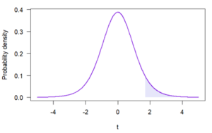
The area, which can be calculated using calculus, statistical software, or reference tables, is equal to .06. Therefore, p = .06 for this sample.
| Distribution | Statistical tests |
|---|---|
| Standard normal (z distribution) | One-sample location test |
| Student’s t distribution | One-sample t test
Two-sample t test Paired t test |
| F distribution | ANOVA
Comparison of nested linear models Equality of two variances |
| Chi-square | Chi-square goodness of fit test
Chi-square test of independence McNemar’s test Test of a single variance |
Probability distribution formulas
| Distribution | Formula | Type of formula |
|---|---|---|
| Binomial | 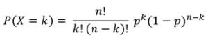 |
Probability mass function |
| Discrete uniform | 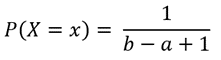 |
Probability mass function |
| Poisson | 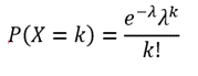 |
Probability mass function |
| Normal | 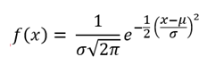 |
Probability density function |
| Continuous uniform | 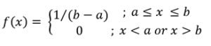 |
Probability density function |
| Exponential | 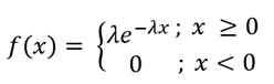 |
Probability density function |
Frequently asked questions about probability distributions
- What’s the difference between relative frequency and probability?
-
Probability is the relative frequency over an infinite number of trials.
For example, the probability of a coin landing on heads is .5, meaning that if you flip the coin an infinite number of times, it will land on heads half the time.
Since doing something an infinite number of times is impossible, relative frequency is often used as an estimate of probability. If you flip a coin 1000 times and get 507 heads, the relative frequency, .507, is a good estimate of the probability.
- What is a normal distribution?
-
In a normal distribution, data are symmetrically distributed with no skew. Most values cluster around a central region, with values tapering off as they go further away from the center.
The measures of central tendency (mean, mode, and median) are exactly the same in a normal distribution.

- What are the two types of probability distributions?
-
Probability distributions belong to two broad categories: discrete probability distributions and continuous probability distributions. Within each category, there are many types of probability distributions.

Sources in this article
We strongly encourage students to use sources in their work. You can cite our article (APA Style) or take a deep dive into the articles below.
This Scribbr articleTurney, S. (June 9, 2022). Probability Distribution | Formula, Types, & Examples. Scribbr. Retrieved October 17, 2022, from https://www.scribbr.com/statistics/probability-distributions/